
Summary #
With the advent of social media, companies soon discovered the ability to influence users’ attention through online marketing communication campaigns. A predictive system capable of determining the impact of individual published posts can give a valuable advantage when deciding to communicate online. Using the data from the Facebook metrics data set, I discovered some interesting insights from the exploratory data analysis and focused on building a predictive tool that can achieve the goal of determining the features that are more likely to cause user engagement.
Introduction #
The data set used in this analysis is the Facebook metrics data set from the UCI Machine Learning web site. A detailed description of the data set and analysis can be found in the 2016 paper by Moro et al., ‘Predicting social media performance metrics and evaluation of the impact on brand building: A data mining approach’. The data set contains posts that were published in 2014 on the Facebook page of a well-known cosmetics company. However, this public dataset only contains 500 of the 790 rows analyzed by Moro et al. As a consequence, the data modeling results of the paper may be hard to replicate. Regardless I give my best attempt at it here.
The paper makes use of seven input features which are used for the modeling, Page total likes, Type, Category, Post month, Post weekday, Post hour and Paid. Page total likes is numerical while the remaining are categorical features. There are also twelve, numerical output features. These are used as performance metrics to gauge the engagement and impressions of the users’ posts. Each of these output performance metric features are individually modeled against the input features, in order to understand what the most predictive metric is. The output features are: Lifetime post total reach, Lifetime post total impressions, Lifetime engaged users, Lifetime post consumers, Lifetime post consumptions, Lifetime post impressions by people who have liked your page, Lifetime post reach by people who like your page, Lifetime people who have liked your page and engaged with your post, Comment, Like, Share and Total interactions. The detailed description of all of these features can be found in the Tables 1. and 2. of the Moro et al. paper, respectively.
Exploratory data analysis #
For the number of posts over the months of the year (Figure 1, left), there are fewer posts in the beginning months of the year and more posts in the spring and early summer, with the exception of a noticeable dip in May, August and September. The month with the most posts coincides with October.
In the center of Figure 1, the number of posts over the days of the week tends to be stable around 70, but it increases noticeably over Friday and Saturday to just over 80.
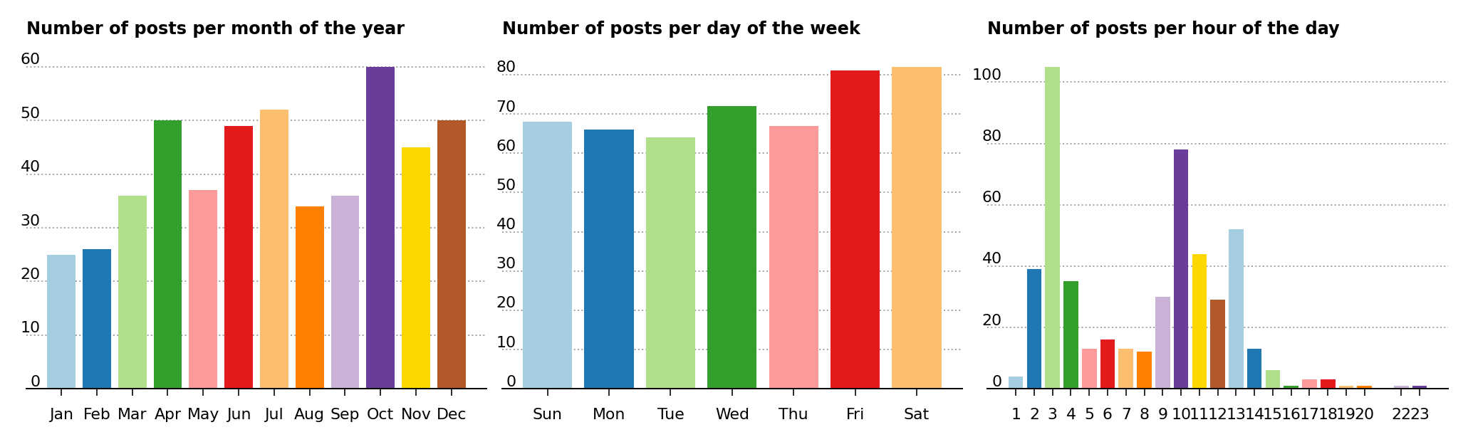
Figure 1 – Number of posts per month of the year (left), number of posts per day of the week (center) and number of posts per hour of the day (right).
For the number of posts made over the hours of the day, shown in left of Figure 1, there are three peaks with the most distinctive one at 3 followed by two secondary peaks at 10 and 13. Unfortunately there isn’t any time zone information available in the data set, so it becomes difficult to establish the precise hour of the day the peaks occur.
Results from the average number of interactions #
For the average number of total interactions per hour of the day (Figure 2, upper left), the error bars were too big to make any statistical distinction except for the measurement at 5. As I mentioned before the lack of time zone information hinders our ability to understand exactly when this measurement occurs during the day. It would be helpful to investigate this measurement to understand why it is so prominent. It is possible that it coincides with the hour the post was initially published in.
In Figure 2 upper right is shown the average number of total interactions per day of the week. There are the days of Tuesday and Wednesday where there is more activity compared to the end of the week, Friday and Saturday. However at the 1 \(\sigma\) error bar level, this is the only statistical distinction that can be made in the plot, as many adjacent bars tend to overlap.
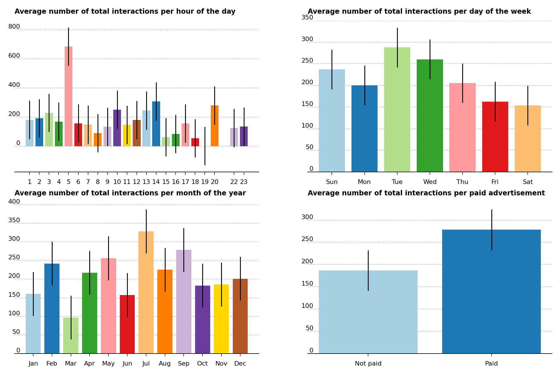
Figure 2 – Average number of total interactions per hour of the day (upper left), average number of total interactions per day of the week (upper right), average number of total interactions per month of the year (lower left) and average number of total interactions of unpaid and paid advertisements (lower right).
Several of the months of the year (Figure 2, lower left) appear to have distinctly more activity than others. July and September appear to have a substantially more activity than other months of the year, such as March and June for example, even taking into account the 1 \(\sigma\) error bars. In general however, the error bars of adjacent months mostly overlap making the statistical separation hard to make.
One interesting insight is the relation between the average number of total interactions and the paid/unpaid status of the post (Figure 4, lower right). The resulting bar plot, with one standard deviation error bars, shows a nearly statistical separation between the average number of total interactions of paid ads versus unpaid ads, which suggests the greater visibility of the former.
Model analysis #
The numerical, input data were normalized using the StandardScaler class, and the categorical, input data were one-hot encoded using the OneHotEncoder class, both from Scikit-Learn. For what concerns the output features, the distributions of the performance metrics contained many outliers. These are easily noticeable with a logarithmic standardized distribution plot of the performance metrics (Figure 3). A Shapiro-Wilk test of normality was performed to test the normality of the distribution of each performance metric. None of the performance metrics passed the test, which denotes a substantial lack of normality in the distributions of all of the performance metrics (see link for Shapiro statistics and p-values results). For the modeling, a threshold of 2 \(\sigma\) was used to remove the outliers of the performance metrics from the data.
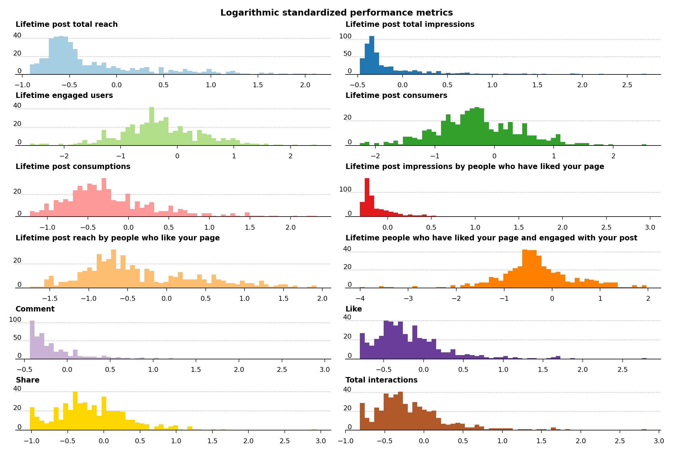
Figure 3 – Distribution of logarithmic standardized performance metrics.
Several machine learning algorithms were used to model the data: Lasso, Random Forest Regressor, Ridge, Stochastic Gradient Descent Regressor and Support Vector Regressor. The root mean squared error (RMSE), the 1 \(\sigma\) standard deviation and the \(R^2\) were calculated for all of the models on each performance metric. The RMSE was calculated from the 10-fold cross validation, using the cross_val_score method and the neg_mean_squared_error scoring parameter. The \(R^2\) was calculated in the same manner but using the r2 scoring parameter.
The stochastic gradient descent regressor achieves the best root mean square error for the Lifetime post impressions by people who have liked your page metric. It was just marginally better than the other machine learning algorithms for this particular feature. However, many of the performance metrics tend to overlap at the 1 \(\sigma\) error bar level. The results of the stochastic gradient descent regressor model calculated against all of the performance metric features are listed in Table 1.
In order to understand if the stochastic gradient descent regressor model can achieve any predictive performance, the \(R^2\) was calculated. It is listed in the last column of Table 1, and its low values reveals the poor predictive performance of the model. Due to the very low values of the \(R^2\), I have avoided any further model calculations of feature importance or permutation importance. It appears that the removal of the data present in the original data set hinders the possibility of improving the model.
| Performance metric | RMSE | SD \((\sigma)\) | Error (%) | \(R^2\) |
|---|---|---|---|---|
| Lifetime post impressions by people who have liked your page | 0.232 | 0.046 | 19.849 | 0.042 |
| Comments | 0.339 | 0.056 | 16.442 | -0.040 |
| Lifetime post total impressions | 0.371 | 0.069 | 18.613 | 0.033 |
| Total Interactions | 0.442 | 0.067 | 15.239 | -0.018 |
| Like | 0.447 | 0.070 | 15.623 | -0.017 |
| Share | 0.473 | 0.062 | 13.112 | -0.051 |
| Lifetime post consumptions | 0.487 | 0.124 | 25.520 | 0.075 |
| Lifetime post total reach | 0.560 | 0.081 | 14.414 | 0.040 |
| Lifetime post consumers | 0.580 | 0.146 | 25.131 | 0.064 |
| Lifetime engaged users | 0.609 | 0.143 | 23.435 | -0.036 |
| Lifetime people who have liked your page and engaged with your post | 0.630 | 0.139 | 22.063 | 0.088 |
| Lifetime post reach by people who like your page | 0.695 | 0.100 | 14.416 | 0.065 |
Conclusions #
An effort was made to analyze the data set and to create a machine learning model to discover the features that are primarily responsible for model prediction. Unfortunately, from the low \(R^2\) of model used for the analysis, there doesn’t seem to be any predictive performance in the model. Consequently, no further investigation into feature importance or permutation importance was attempted. However from the exploratory data analysis, we can notice some insights into the average number of total interactions and the number of posts over the hours of the day, the days of the week and the months of the year.
You are more than welcome to take a look at the code in my GitHub repository. For the analysis, the following software packages were used: Scikit-Learn (version 1.2.2), pandas (version 1.5.3), matplotlib (version 3.7.1) and NumPy (version 1.24.2).
UPDATE (2023-03-27): I’ve updated the analysis by using logarithmic standardized performance metrics, using the latest version of Scikit-Learn (version 1.2.2) as listed above.